The Attribution Continuum: How Shapley Divides the Credit
The Math, the Code, and the Limits


What brought us to Shapley
In the previous post I described attribution as a continuum, from heuristic rules at one end to causal methods at the other, and made the case that heuristics are often the right choice, particularly for teams without the data to reliably support anything more complex. I also introduced Ron Berman’s 2018 Marketing Science paper, Beyond the Last Touch, which gives us a specific reason to graduate from heuristics.
Berman showed that last-touch attribution creates an incentive problem. When actors know they benefit from showing up at a specific position in the journey, they optimize for that position rather than for the business outcome. He studied this in the context of online advertising, but the intuition likely applies more broadly; when an attribution rule rewards position, people may start optimizing for the rule itself rather than the outcome it was meant to measure. Berman found that Shapley largely addresses this because it assigns credit based on each channel’s average marginal contribution across all possible combinations, making credit allocation less directly tied to any single journey position.
In this post I break down exactly how Shapley works, walk through the mechanics with a concrete example, and give you the code to run it yourself.
How Shapley divides the credit
Shapley values come from cooperative game theory, a branch of mathematics concerned with how to fairly divide a reward among players who contributed to it together. Think of a closed deal as the reward and each sales (and marketing) channel as a player that contributed to winning it. The question cooperative game theory asks, and the question Shapley answers, is how to divide that reward fairly.
What heuristics do is pick a rule and apply it uniformly regardless of what the data says. Shapley takes a different approach. For each channel, it looks at every possible combination of channels that appeared across your pipeline and asks: how did win rates differ when this channel was part of the mix versus when it was not?” The answer to that question, summed across all combinations and weighted proportionately, becomes that channel’s credit weight.
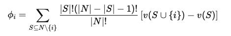
The formula below, developed by Lloyd Shapley in 1952, is the engine behind that calculation. It may look intimidating at first glance, but what it is doing is straightforward. I will walk through each part using a concrete example with four channels: ABM Ads, Webinar, Executive Briefing, and Sales Calls.
Our hypothetical dataset contains both closed-won and closed-lost opportunities. Each row is one account. Each channel is a binary column, present or absent. The outcome is 1 for closed-won, 0 for closed-lost. Because each channel is either present or absent, four channels produce 2^4 = 16 possible combinations. I will call each combination a coalition. For each coalition, we estimate the win rate among accounts that received exactly that combination of channels. Those win rates are what the formula works with.
Two things worth flagging before we work through the example. Standard Shapley treats each channel as present or absent. It does not account for frequency or the order in which channels appeared, both of which almost certainly matter in practice. I will address those limitations in future posts covering ordered Shapley and Markov chain attribution. The win rates in the example below are also illustrative. In practice they would come from your own pipeline data.
Part one: the marginal contribution
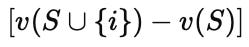
The first part of the formula measures how much the win rate changes when a channel is added to a coalition that does not already include it. For example: if accounts that received only Sales Calls had a win rate of 0.30 and accounts without any channels at all had a win rate of 0.05, the marginal contribution of Sales Calls entering an empty coalition is 0.30 - 0.05 = 0.25. Shapley repeats this calculation for every channel across every possible coalition, building up a complete picture of each channel’s contribution under every scenario. You will see this in practice shortly when we walk through a complete example.
Part two: the weighting
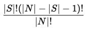
Because Shapley evaluates every possible coalition, the second part of the formula provides a principled way to average those marginal contributions together. We showed earlier that the marginal contribution of Sales Calls entering an empty coalition is 0.25. Now consider the other extreme: when Sales Calls is added to a coalition that already contains ABM, Webinar, and EBC, the win rate goes from 0.32 to 0.65, a marginal contribution of 0.33. These two observations should not necessarily carry equal weight in the final average.
The weighting formula handles this. With four channels |N| = 4, the weights by coalition size |S| are:
|S| = 0 (no other program present): = 0!(4 - 0 - 1)! / 4! = 0!*3! / 4! = 1*6 / 24 = 1/4
|S| = 1 (one other program present): 1!*2! / 4! = 1*2 / 24 = 1/12
|S| = 2 (two other programs present): 2!*1! / 4! = 2*1 / 24 = 1/12
|S| = 3 (three other programs present): 3!*0! / 4! = 6*1 / 24 = 1/4
Notice that size 0 and size 3 carry the same weight, and size 1 and size 2 carry the same weight. This is by design. Shapley is built around a symmetry principle; a channel entering an empty coalition and a channel entering a nearly full coalition are both extreme scenarios and are treated equally. This is one expression of why Shapley is harder to game than heuristics that explicitly reward position.
Part three: the sum

The third part of the formula, is the instruction to take the product of each marginal contribution and its corresponding weight from parts one and two, and sum those products together. That sum is ϕi, the Shapley value for channel i.
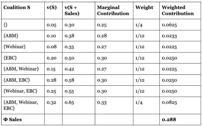
To make this concrete, below is the full calculation for Sales Calls across all eight coalitions that do not already include it. For this example, treat v(S) and v(S + Sales) as given. In practice these come directly from your pipeline data, and the Python code later in this post shows exactly how to calculate them.
Running the same process for ABM Ads, Webinar, and Executive Briefing produces the following:
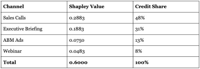
Sales Calls earns the largest weight and Executive Briefing the second largest. Sales Calls produces the largest marginal lift across every coalition it enters, with a minimum contribution of 0.25 regardless of what other channels are present. Executive Briefing is the only other channel that contributes meaningfully on its own, adding 0.15 in win rate above the baseline before any other channel is present. ABM and Webinar earn smaller weights because their absolute marginal contributions are lower across all coalitions.
Quick reminder: these weights are a function of the win rates in this specific example. Run this on your own data and the numbers will look different. That is the point.
Running Shapley yourself
The dataset attached to this post contains 1,200 accounts. Each row shows which of the four channels, ABM, Webinar, Executive Briefing, and Sales Calls, touched the account during the sales cycle, and whether the relevant deal became closed won or closed lost.
The full notebook is available here: [Google Colab link]. A Google Colab notebook is a free, browser-based environment where you can run Python code without installing anything on your computer. You open it like a webpage, run the code one cell at a time, and see the results instantly. If you have never written Python before, do not let that stop you. AI tools like ChatGPT can explain any line of code you do not understand, help you modify it for your own data, and fix errors when they come up. Running code has never been more accessible than it is right now, and a Colab notebook is the best place to start.
Download the dataset, open the notebook, and run each cell in order from top to bottom by clicking the play button on the top left corner of each cell. After running the first cell, scroll to the bottom of that cell and click “Choose Files” to upload the dataset. The screenshot below shows exactly where to look.
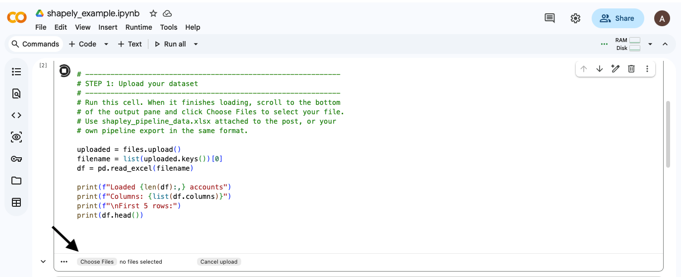
The notebook walks through four steps: upload your file, define your channels, calculate win rates for each channel combination from the raw data, and run the Shapley formula. Once you have it working on the synthetic data provided, you can feel free to try it on your own data. If you want to adapt the code, whether that means adding more channels or changing the outcome definition, paste the code into ChatGPT and ask it to help you make the change.
If you want to go deeper on how sample size of each channel combinations affects the reliability of win rate estimates, OpenStax's chapter on confidence intervals for proportions is a good place to start: [link].
A note on computation and ordering
The formula I implemented in the notebook works cleanly for a small number of channel categories, but it has two limitations.
The first is computational. As the number of channels grows, the number of coalitions grows exponentially. With 4 channels you have 2^4 = 16 coalitions. With 10 you have 2^10 = 1,024. With 30 you have 2^30 = over a billion. Every channel you add doubles the number of coalitions the formula needs to evaluate.
The second is that standard Shapley is order-agnostic. It treats a channel that appeared in month one the same as one that appeared in month twelve, as long as their marginal contributions are equal. In B2B enterprise that is a real limitation. SDR outreach before an executive briefing before a demo can be a meaningfully different journey than the same three channels in a different order.
Zhao, Mahboobi & Bagheri tackled both limitations in their 2018 paper, Shapley Value Methods for Attribution Modeling in Online Advertising. They developed a more efficient version of the formula and an ordered variant that accounts for the sequence in which channels appeared. I will cover both in a future post.
Why Shapley still isn’t causal
Shapley is fair in a specific mathematical sense: every channel’s credit reflects its average marginal contribution across every possible combination of channels. That is not the same thing as causal. The formula distributes credit based on observed win rates across channel combinations, but those combinations did not occur randomly. In some companies, Enterprise Events for example get assigned primarily to large accounts that were already likely to close. In that scenario, Shapley will give Enterprise Events a large credit weight because the win rate is higher when Enterprise Events is in the coalition. Although that weight is fair under Shapley’s axioms, it is confounded by the fact that high-propensity accounts got the channel in the first place.
Shapley cannot see the difference between a channel that drove conversion and a channel that was assigned to accounts that were already going to convert. That distinction requires thinking causally about how channels get assigned to accounts, not just what the win rates look like after the fact. We will cover that in a future post.
Where Shapley sits on the attribution ladder
Shapley is the first stop past heuristics, but it is not the destination. Through this series I want to walk up the full attribution ladder one rung at a time. Here is how I think about it.
Rung 1 (Heuristics): Last-touch, first-touch, U-shape, full-path. Cheap, fast, often the right choice early on. Covered in post 1.
Rung 2 (Descriptive attribution: Standard Shapley): Fair credit allocation across channels that touched a deal, defensible under cooperative game theory axioms. Covered in this post.
Rung 3 (Descriptive attribution with sequence): Adds order to the picture, since SDR outreach before a demo is a different journey than the reverse. Two foundational methods address this directly: ordered Shapley and Markov chain attribution. At the more advanced end, deep learning models like LSTMs can learn complex sequential patterns directly from journey data. It is worth noting that LSTMs and similar models are not a separate rung on the ladder. They are an estimation engine that can power methods across multiple rungs, from sequence-aware attribution at Rung 3 to causally-corrected approaches at Rung 4. We will cover the foundational methods first and return to how advanced models fit into the full picture later.
Rung 4 (Causally-corrected attribution): Distinguishes channels that drove conversion from channels that were assigned to accounts already likely to convert. It corrects for selection bias in your historical data, giving you a more honest picture of past channel impact. But it is still a backward-looking measurement. It tells you what worked given the mix you ran, not what would happen if you changed it.
Rung 5 (Forward-looking budget optimization): Rungs 1 through 4 are all backward-looking. Even causally-corrected attribution tells you what drove conversion given the programs you ran. It does not tell you what would happen if you shifted budget, ran one more field event, or cut a program entirely. Answering those questions requires understanding how outcomes respond at the margin as spend changes, how returns diminish as you do more of the same thing, and how some programs generate carryover effects that show up in future quarters rather than the current one. A 2018 Journal of Marketing Research paper by Peter Danaher and Harald van Heerde made this case precisely: attribution estimates are backward-looking and cannot reliably guide forward-looking allocation decisions. Tools like Meta's Robyn and Google's Meridian attempt to model these dynamics directly. Whether and how they apply in enterprise B2B contexts, where programs are discrete and infrequent rather than continuous, is something we will work through later in the series.
We have now covered rungs 1 and 2. We will cover the remaining rungs in future posts.